Combining Optimization with Machine Learning for better Branch & Bound

Optimization problems exist all around us in various forms. They come in all scales, from a manager assigning tasks to employees in the best possible way to a logistics company  planning its vehicle routes to save fuel.
These are all optimization problems. Solving these problems fast and accurately is important for businesses, but it’s often challenging. That’s because these problems are combinatorial in nature, which means they involve many different combinations, and trying them all would take a large amount of time.

 Branch-and-Bound - A Classic Optimization Algorithm

Branch-and-Bound (BnB) is one of the most common ways to solve these kinds of problems. Think of a big decision tree where each point (called a node) is a partial solution and it is necessary to explore different paths to find the best complete solution. Instead of exploring every possible path, BnB eliminates paths that are unlikely to lead to the best solution, and saves a lot of time and computational effort. At each node, the algorithm makes two key decisions:

1. Should it keep exploring this path? (Bounding step)
   
2. If yes, which variable should it branch on next? (Branching step)
   

This second decision of selecting the variable to branch on has a huge impact on how efficiently the algorithm finds the optimal solution. 

Strong Branching for Branching Decisions

One way to decide which variable to branch on is called strong branching. Strong branching tries out each possible option temporarily. For each variable that can be branched on, the algorithm:

• Pretends to branch on it (without fully committing), by
  
• Solving the relaxed version of the problem for each branch (left and right),
  
• Measures how much the objective value improves or how much the objective bounds of the problem are tightened.
  

It then picks the variable that gives the strongest improvement, and eliminates all other branches from further exploration, which makes it very accurate and effective at reducing the search space. It gives high-quality decisions that usually lead to quality solutions, but it’s also very slow and expensive, especially for large problems, and can’t be used all the time during solving .

Pseudocost - A Faster Alternative

Since strong branching is slow to use throughout the entire solve, traditional BnB algorithms use a faster alternative called pseudocost branching. Here’s how it works:

• The algorithm keeps track of how effective each variable was in past branching decisions and how much the objective improved when it was branched upon.
  
• Over time, it builds up average scores (called pseudocosts) for each variable as their domains are tightened.
  
• The highest pseudocost scores are used to determine which variable should be evaluated next.
  

This method is much faster because it doesn’t simulate or test each integer infeasible variable like in strong branching. But, it comes with a trade-off; when there is not much historical branching data collected,  pseudocost estimates can be unreliable and can lead to poor branching decisions, especially in the early stages of the BnB process.

Can Machine Learning Do Better?

We’re exploring whether machine learning (ML) can improve how BnB decides which variable to branch on. We call this  ML-BVS, which stands for: Machine Learning-Branch Variable Selection. The idea is simple: Use ML to learn from good branching decisions (using real data), and then use that learning to make better decisions  for branching on the variables in the  problem.

How Our ML-BVS Process Works

We’ve designed a process with three main steps:

1. Data Collection using Strong Branching

We first collect training data using  strong branching. As stated earlier, Strong branching is slow and expensive, we only use it in the training phase to generate high-quality data. We record:

• Which variable was best to branch on .
  
• A total of 50 + unique features of the variables (like pseudocosts, objective coefficients, constraint-related statistics, etc.) for the data collection process and ML models to train from. 

2. Model Training

We feed this data into a machine learning model, which looks for patterns and combines the features that lead to the best branching decisions. We tested different  ML models like:

• Random Forests (which use many decision trees to make predictions)
  
• XGBoost (a powerful boosting algorithm that combines many weak learners to improve inference accuracy)
  
• SVMs (Support Vector Machines, which finds an optimal decision boundary that separates (classifies) low and high quality branching decisions)
  

3. Real-Time Prediction During Optimization

We freeze the model after training, which means we lock in what it has learned and only use it to make predictions (i.e. infer the next branching variable), to eliminate need for costly strong branching. The ML model predicts the best branching variable at each  node in the BnB tree during the process of solving the optimization problem.

Here’s how that looks in practice:

• For every candidate variable in a layer of the BnB tree, we collect the same set of features at every node.
• The trained model looks at these features and gives each variable a score or ranking for how well the improvement in the objective could be if we branched on it.
• We choose the variable that the model suggests, evaluate that node using the LP solver and then move on to the next iteration of branching.
  

Testing

We did controlled experiments to test the performance of the ML models as a branching variable selection strategy on various benchmark problems from the MIPLIB2017 dataset. Specifically, we asked:

• Can the model replicate the branching decisions that a traditional pseudocost heuristic would make?
  
• Are the decisions and outcomes consistent and stable from run-to-run and between problem instances?
  
• Can the model outperform pseudocost by finding a better solution faster?

Results: How Does ML Compare to Traditional Pseudocosts?

For testing, and to answer these questions, we ran experiments on several benchmark problems from MIPLIB2017. Each problem was solved using four different branching strategies:

• Random (as a baseline)
  
• Pseudocost (traditional method)
  
• SVM implemented through PairwiseTransformSGD (stochastic gradient descent)
  
• Random Forest Classifier Model (an ensemble ML model using many weak decision trees)
• Each method was allotted the same maximum solve time of 1 hour to make the comparison fair.

‍

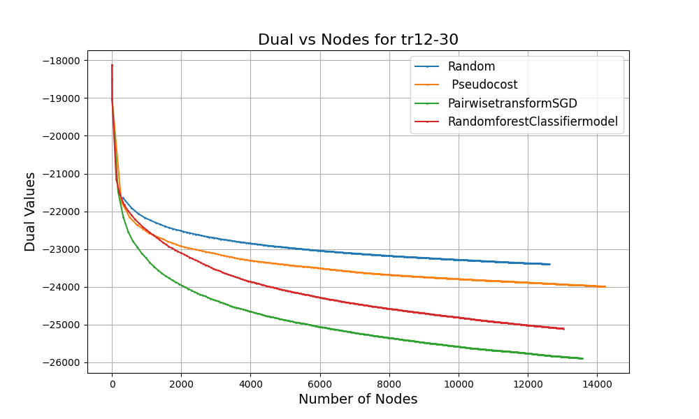
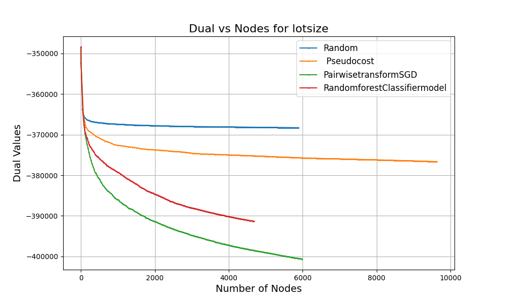
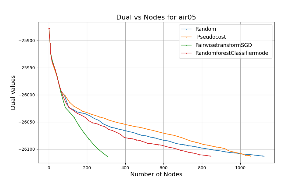
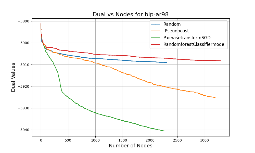
These graphs show some of the results that we observed. At every step in the optimization, we tracked:

• Dual values: These tell us how tight the lower bound of our optimization problem is. Better (i.e. higher for maximization, lower for minimization) dual values mean we converging to the optimal solution.
  
• Number of nodes explored: This metric helps us quantify the amount of computational effort used and node throughput. The ratio of the final dual value to total number of node evaluations provides a measure of computational efficiency for each method within the allowed 1 hour solve timelimit.
• We fixed the primal values to the objective value of the optimal solution, which were known to us ahead of time, and set the optimality gap ( gap between dual and primal ) threshold to less than 1% as our stopping criteria. This way, we could focus only on which method was better at improving the dual value by observing the reduction in the dual per number of node evaluations.

In the plots:

• The X-axis shows Number of nodes explored
• Y-axis shows Dual value at that point
• Each colored line represents a different branching variable selection method

The goal is to shrink the dual bounds faster - i.e. steeper curves in the plot (for minimization problems) - in the fewest number of node evaluations. Each curve on the graph shows how the dual value improves as the MIP solver traverses the branch and bound tree. You will notice:

• Random strategies performed poorly, highlighting the value of intelligent branching strategies.The gap of less than 1% was consistently reached fastest by ML-based methods in several cases, demonstrating that good branching decisions significantly reduce computational effort.
• ML BVS strategies achieve better dual bounds with fewer nodes, showing they’re choosing smarter branching variables.
  
• The ML curves are shorter because ML-based branching has slightly lower node throughout (due to the extra time spent evaluating the model), but they still beat pseudocosts by reaching the target gap faster.

These results confirm our hypothesis: machine learning can help branch-and-bound solvers make smarter decisions, especially in the early stages of solving complex problems.

While pseudocosts are calculated during the solve process and require branching multiple times on the same variable to be useful, ML models are pre-trained on high-quality strong branching data at the onset  and can yield good decisions even early on in the branch and bound process. This provides evidence that choosing the right ML model for branching variable selection leads to tighter bounds and reducing node exploration times.

What’s Next?

We will continue working on:

• Identifying richer input features to improve the predictive power of the ML models.
  
• Analyzing different ML models to identify the most performative ones, including the kinds of the problem instances they perform best on.
  
• Testing our approach on larger, and harder problems to see how well these branching variable selection strategies scale.

We’re excited to continue this exploration, and we’ll keep sharing what we learn.